Neural Network Taxonomy:

This section shows some examples of neural network structures and the code associated with the structure. First, a couple examples of traditional neural networks will be shown. This form of network is useful for mapping inputs to outputs, where there is no time-dependent component. In other words, the knowledge of past events is not predictive of future events. The next section shows various forms of recurrent networks, which attempt to retain a memory of past events as a guide to future behavior.

Traditional Neural Networks

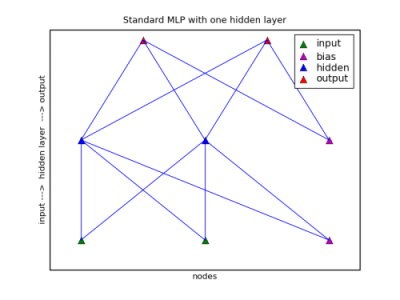
Multilayer Perceptron with One Hidden Layer

This standard form of neural network has one hidden layer between the inputs and the outputs. In the following code in all of these examples, the initial imports of the modules are assumed.

#   Standard MLP with one hidden layer
input_nodes = 2
hidden_nodes = 2
output_nodes = 2

net = NeuralNet()
net.init_layers(input_nodes, [hidden_nodes], output_nodes)
net.randomize_network()

Note that the number of hidden nodes is in a list, even if there is only one hidden layer.

Multilayer Perceptron with Two Hidden Layers

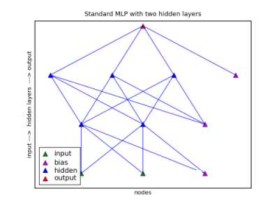The next form is the same as the first, with the exception that there are two layers.

#   Standard MLP with two hidden layers
input_nodes = 2
hidden_nodes1 = 2
hidden_nodes2 = 3
output_nodes = 1

net = NeuralNet()
net.init_layers(
    input_nodes,
    [hidden_nodes1,
    hidden_nodes2],
    output_nodes)

net.randomize_network()

Recurrent Networks

The following network types are forms of recurrent networks. Recurrent networks use a structure that retains previous values in an attempt to model a memory of past events. While normally a network feeds forward values from lower layers to upper layers, a recurrent network also has returning links to additional copy or context units on the same or lower layers.

The execution sequence of the network becomes:

• feed-forward
• back propagation, if in learning mode
• feed back values from some nodes to copies
• acquire the next set of inputs
• repeat

The copies at time t always have the values of the source nodes at t-1. There is also no reason why copies cannot be made of copies, so that some copies can contain t-2, t-3, and so on.

There are various network forms; some will retain copies of previous input nodes, hidden nodes, or output nodes. There are such factors as whether the source value replaces, or adds to a copy value, or some combination of both. These additional nodes have been given various names, such as context and state as a way of describing their role. In this description and in the software classes, the nodes are referred to as copy nodes to reflect the functional roles.

One thing to note regarding any recurrent network form: When using the learn function, the random_testing variable should always be set to False. If set to True, any value from using recurrent forms would be lost, since the sequence would be non-patterned.

In the charts to follow, the feed-forward connections are shown on the charts, the connections linking back to the copy nodes do not. By each copy node, however, the source of the values is shown.

Elman Simple Recurrent Network

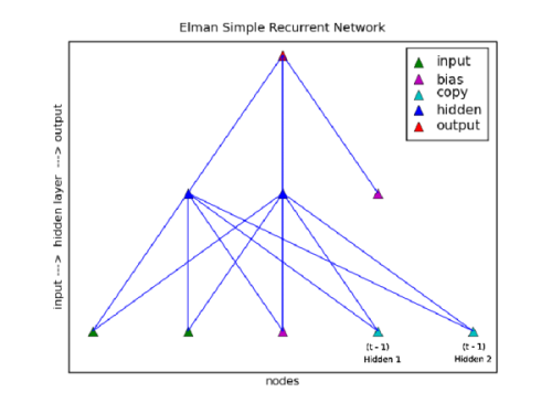The Elman Simple Recurrent Network approach to retaining a memory of previous events is to copy the activations of nodes on the hidden layer. In this form a downward link is made between the hidden layer and additional copy or context units (in this nomenclature) on the input layer. After feeding forward the values from input to output a copy of the activations of the hidden layer replaces the value in the copy or context nodes. So, the context nodes at time t have the values of the hidden nodes from at t - 1. Finally, the activation type of the copy nodes are always 'linear'.

#   Elman Simple Recurrent Network
input_nodes = 2
hidden_nodes = 2
output_nodes = 1

net = NeuralNet()
net.init_layers(
    input_nodes,
    [hidden_nodes],
    output_nodes,
    ElmanSimpleRecurrent())

net.randomize_network()

Jordan Style Recurrent Network

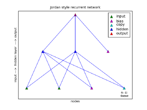A Jordan style recurrent network differs from an Elman style in a couple ways. First, the links are made from the output layer, not the hidden layer. Second, the manner in which the copies are made is different. When the Elman SRN copies a value from a hidden node, the value in the copy node is replaced, the Jordan recurrent network adds uses a factor to reduce the current value in the copy node and then adds the new copy value to the value in the copy node.

New copy value = Output Activation value + Existing Copy Value * Weight Factor

The following code shows an example of initializing this style of network.

#   Jordan style recurrent network
input_nodes = 2
hidden_nodes = 2
output_nodes = 1
existing_weight_factor = .7
net = NeuralNet()

net.init_layers(
    input_nodes,
    [hidden_nodes],
    output_nodes,
    JordanRecurrent(existing_weight_factor))

net.randomize_network()

Note that the existing weight in the copy node in this case is reduced to 70%. Then the new copy value is added to it. In this style network, the copy node has a linear activation.

New Copy value = Output Activation value + Existing Copy Value * Existing Weight Factor

NARX (Non-Linear AutoRegressive with eXogenous inputs) recurrent network

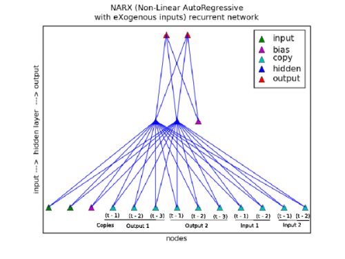
Another approach to recurrence is NARX (Non-Linear AutoRegressive with eXogenous inputs) recurrent network. This form with the mellifluous name can take copies from the output and input layers. Multiple levels of copies can be maintained, such as times t-1, t-2, t-3, and so on. In this network's nomenclature, the number of copies are referred to as the 'order'.

The transfer of the copy value in this case replaces the previous value. In addition, a weighting factor is applied to a transfer so that a copy value is attenuated at each level.

New Copy value = Output Activation value * Incoming Weight Factor + Existing
Copy Value * Existing Weight Factor

The chart shown to the right illustrates the additional copy nodes. Note the multiple copies for both the output and the inputs.

#   NARXRecurrent
input_nodes = 2
hidden_nodes = 2
output_nodes = 2

output_order = 3
incoming_weight_from_output = .6
input_order = 2
incoming_weight_from_input = .4

net = NeuralNet()
net.init_layers(input_nodes, [hidden_nodes], output_nodes,
        NARXRecurrent(
            output_order,
            incoming_weight_from_output,
            input_order,
            incoming_weight_from_input))

net.randomize_network()

Other Examples

This is an example of how to use the RecurrentConfig class to create a specific structure. The use of this class is a convenience, greater control and greater specificity will be achieved by modifying the network directly. However, the capabilities of the class might be sufficient for many needs.

Suppose you needed a network that had the combined capabilities of both Elman and Jordan style networks. One option would be to use the following:

input_nodes = 2
hidden_nodes = 2
output_nodes = 1
existing_weight_factor = .7

net = NeuralNet()
net.init_layers(
    input_nodes,
    [hidden_nodes],
    output_nodes,
    ElmanSimpleRecurrent(),
    JordanRecurrent(existing_weight_factor))

net.randomize_network()

Adding multiple RecurrentConfig classes to the network is an accretive process. Each one adds copy nodes to the network. In this case, there would be one copy node that would receive source values from the output node, and two copy nodes that would receive values from the hidden nodes. In this example, the updates to those copy nodes would be handled in the manner of the respective class. If you need a different strategy, you can build your own.

Build Your Own RecurrentConfig class

Another approach would be to subclass RecurrentConfig into whatever configuration you needed. For example, suppose you wanted to use a history of one of your input values, but no others. For purposes of this example:

• the first input is maintained in a history

• every copied value included 70% of the copied value and 30% of the existing copied value

• specify an arbitrary level of copies

• linear activation
• copy nodes placed on the input layer
• connects to the hidden layer
• fully connected to the hidden layer

Most of the defaults for the class are kept the same. Only a few variables need to be changed. Below you can see how those changes are made. All the defaults are shown here for completeness, but when making a new class, of course, you only need to include the variables that are different from the base class.

In this case we have changed the incoming_weight and existing_weight variables, and added copy_levels as an input. The only other thing that is needed is to provide a mechanism for the selection of the right input.

class MyNewRecurrentClass(RecurrentConfig):
    def __init__(self, copy_levels):
        RecurrentConfig.__init__(self)
        self.source_type = 'a'
        self.activation_type = 'linear'
        self.incoming_weight = 0.7
        self.existing_weight = 0.3
        self.connection_type = 'm'
        self.copy_levels = copy_levels
        self.copy_nodes_layer = 0
        self.connect_nodes_layer = 1

    def get_source_nodes(self, neural_net):
        """
        This function selects the first input node.

        """

        return neural_net.layers[0].get_nodes('inputs')[0]

By defining the get_source_nodes function, you specify what source nodes are used. In this case, we are getting the nodes from the input layer, layer 0. From the layer, only nodes that are of type 'input' are selected. This enables screening out bias nodes and other copy nodes. Finally, it selects only the first node of the input nodes.

Now, we can put this class into play in a similiar fashion to the other examples:

input_nodes = 2
hidden_nodes = 2
output_nodes = 1
existing_weight_factor = .7
copy_levels = 10

net = NeuralNet()
net.init_layers(
    input_nodes,
    [hidden_nodes],
    output_nodes,
    MyNewRecurrentClass(copy_levels))

net.randomize_network()