Neural Network Tutorial:

Installation

The quickest way to install is with easy_install. Since this is a Python library, at the Python prompt put:

easy_install pyneurgen

This section will go through an example to get acquainted with the software. To illustrate what is happening here, we will also use a separate Python software package called matplotlib. If you are not already acquainted with the package, you will find that it is very helpful for 2d plotting and well worth adding to your system. It can be gotten at http://matplotlib.sourceforge.net

We will start with a simple neural network that calculates a sine related function with a slight random component to make it slightly more interesting:

The first step is import the modules, and initialize the data.

import random
import math

import matplotlib
from pylab import plot, legend, subplot, grid, xlabel, ylabel, show, title

from pyneurgen.neuralnet import NeuralNet
from pyneurgen.nodes import BiasNode, Connection

Inputs and Targets

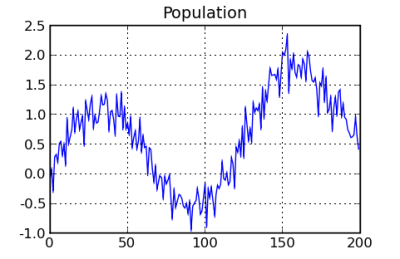
Now, we will set up inputs and targets. The following code just creates a list of inputs and targets. The random component is added as an input to make the overall result a little more interesting or challenging. The network must learn to ignore the random input and will just have to live with trying to understand the random component in the target data. One important thing to remember is that the input should be normalized so that it is in the vicinity of -1 to +1. That helps to avoid overflow issues related to weights trying to adjust for errors. This package does not normalize data automatically, because it should be done individually for each project. For example, if timeseries data was normalized automatically, it might have a different starting point between testing and putting the neural network into production. The chart at the right shows the data that is created.

The population is built and then sorted randomly. The data is placed into the inputs and targets for the neural net. The last 20% of the data will be used for testing.

#   all samples are drawn from this population
pop_len = 200
factor = 1.0 / float(pop_len)
population = [[i, math.sin(float(i) * factor * 10.0) + \
                random.gauss(float(i) * factor, .2)]
                    for i in range(pop_len)]

all_inputs = []
all_targets = []

def population_gen(population):
    """
    This function shuffles the values of the population and yields the
    items in a random fashion.

    """

    pop_sort = [item for item in population]
    random.shuffle(pop_sort)

    for item in pop_sort:
        yield item

#   Build the inputs
for position, target in population_gen(population):
    pos = float(position)
    all_inputs.append([random.random(), pos * factor])
    all_targets.append([target])

Network Structure

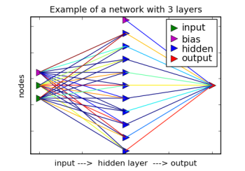
After importing and instantiating the main class NeuralNet called net. Then, it specifies a network structure of 2 inputs, 1 hidden layer of 10 nodes, and finally, 1 output. Note that this hidden layer is a list and can contain any number of hidden layers, although more than two hidden layers would be unusual.

The default values initiate a network structure with a set of network nodes. Each node is fully connected to the layer below. In addition, the learn rate is set to .20. That means that 20% of the error between each instance of target and output will be communicated back down the network during training. The next step in the process is to randomize the weights of each connection. Without starting random values, the process of search is not able to differentiate one set of nodes from another.

net = NeuralNet()
net.init_layers(2, [10], 1)

net.randomize_network()
net.set_halt_on_extremes(True)

#   Set to constrain beginning weights to -.5 to .5
#       Just to show we can
net.set_random_constraint(.5)
net.set_learnrate(.1)

Now that the network structure is created, the inputs and targets are loaded into the system.

net.set_all_inputs(all_inputs)
net.set_all_targets(all_targets)

The first 80% of the data will be used for learning and the rest will be set aside for testing. We will skip validation testing for these purposes. The net object is notified of that in the following:

length = len(all_inputs)
learn_end_point = int(length * .8)

net.set_learn_range(0, learn_end_point)
net.set_test_range(learn_end_point + 1, length - 1)

The activation types for a network default to 'linear' for the input layer, 'sigmoid' for the hidden layers, and 'linear' for the output. For this example, the hidden layer will be set to 'tanh'. Layers are organized in a list with the input layer as 0, hidden layers 1 and above, ending in the output layer as the last.

net.layers[1].set_activation_type('tanh')

At this point we have the data loaded, the network structure defined and ready. We can now start the network learn process which sets the appropriate weights for each connection. This process will be run in this case with 10 trips through the data. Each trip is called an epoch. There is also an option of loading in the data in a random fashion.

net.learn(epochs=125, show_epoch_results=True,
    random_testing=False)

With learning complete, it is time to test and evaluate the results.

mse = net.test()

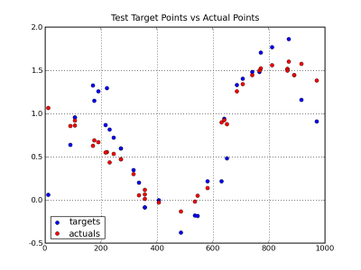
To view the results we will use some matplotlib charts. The first chart compares the test versus actual for the 20% that was tested. You can see that the general shape of the population shows in the sample. In addition, the actual values are mostly representative of the target values. Because of the random component of the population data, there is no expectation that it would exactly match.

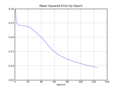
The second chart shows the mean squared errors for each epoch. Ideally, the progress of reducing error should be steadily downwards.

Below, is the code used to generate the charts:

test_positions = [item[0][1] * 1000.0 for item in net.get_test_data()]

all_targets1 = [item[0][0] for item in net.test_targets_activations]
allactuals = [item[1][0] for item in net.test_targets_activations]

#   This is quick and dirty, but it will show the results
subplot(3, 1, 1)
plot([i[1] for i in population])
title("Population")
grid(True)

subplot(3, 1, 2)
plot(test_positions, all_targets1, 'bo', label='targets')
plot(test_positions, allactuals, 'ro', label='actuals')
grid(True)
legend(loc='lower left', numpoints=1)
title("Test Target Points vs Actual Points")

subplot(3, 1, 3)
plot(range(1, len(net.accum_mse) + 1, 1), net.accum_mse)
xlabel('epochs')
ylabel('mean squared error')
grid(True)
title("Mean Squared Error by Epoch")

show()