Genetic Neural Hybrid Tutorial:

This tutorial presents a hybrid use of grammatical evolutionary techniques with a neural network. Just as in the tutorial for grammatical evolution, there are definitions of variables in a BNF context that the program will use to build a neural network. In this example as well, there is a starting point with a program that is partially built. This partially built program implements a machine building of the network component by component, hence more code than the neural network tutorial.

Similarly to the neural network tutorial, this tutorial assumes that you have matplotlib installed as well.

The Objective

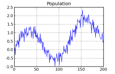
Given a randomized sine wave as in the purely neural networks example, develop a neural network, that is able to discern the pattern.

The means to achieving the objective specified via the choices in the BNF are:

• Determine an appropriate number of hidden nodes.
• Define the activation type
• Define the connection weights
• Determine a learning rate

In this case, the number of hidden nodes is determined by the genotype. Then, once defined by the genotype, the type of activation is also set by the genotype. Then, connections are made, or not, depending upon the genotype. And, connection weights are assigned by the genotype.

For this example, the search used by grammatical evolution defines the structure and activation functions. The weights might be adjusted via the learning process, or not, depending upon the value of <epoch>. If it is zero, then learning is skipped, and an evaluation is made on the basis of the starting weights alone.

Finally, the network model is saved to disk.

Backus-Naur form

The BNF in this case contains variables related to the structure of the network, such the maximum number of hidden nodes, and node types. The number of input and output nodes are placed in here as well, but only to generalize the <S> starting point.

There is also a provision for building a filename for each network model. Since presumably the point of finding the best network model would be to reuse it, there needs to be provision for instantiating that model with all of the right structures and parameters. There is also a variable <model_name>. This takes the <member_no>, or position within the population and combines with a prefix and suffix, suitable for a filename. <member_no> is loaded in the local BNF for each genotype automatically. In the <S>, there is a statement saving each model to disk. If you did not want to save files, you could also use the result of net.output_values() and project that somewhere. Here is the BNF with the exception of <S> defined:

bnf =   """
<model_name>        ::= sample<member_no>.nn
<max_hnodes>        ::= 40
<node_type>         ::= sigmoid | linear | tanh
<positive-real>     ::= 0.<int-const>
<int-const>         ::= <int-const> | 1 | 2 | 3 | 4 | 5 | 6 |
                        7 | 8 | 9 | 0
<sign>              ::= + | -
<max_epochs>        ::= 1000
<starting_weight>   ::= <sign> 0.<int-const> | <sign> 1.<int-const> |
                        <sign> 2.<int-const> | <sign> 3.<int-const> |
                        <sign> 4.<int-const> | <sign> 5.<int-const>
<learn_rate>        ::= 0.<int-const>
<saved_name>        ::= None

This <S> is much more structured than the grammatical evolution tutorial. We want specific choices to be made, but need a working network model as an end result. The first few lines import and instantiate the model, and then structure the input layer. Then, a choice is made by the genotype regarding the number of hidden nodes. Those decisions are made by using preprocessing. At runtime, with the structure of the network defined, the choices for what hidden node types, connections, and starting weights are made.

Next, the input data and targets are defined and loaded. In this case, the point of the model is to predict a probabilistically varied sine wave.

Finally, the learning mode is used, to build the best weights given the network structure. The mean-squared error of the test function is calculated and used as a fitness value, and the model is saved.

<S>                 ::=
import math
import random

from pyneurgen.neuralnet import NeuralNet
from pyneurgen.nodes import Node, BiasNode, CopyNode, Connection
from pyneurgen.layers import Layer
from pyneurgen.recurrent import JordanRecurrent

net = NeuralNet()
hidden_nodes = max(int(round(<positive-real> * float(<max_hnodes>))), 1)

net.init_layers(len(self.all_inputs[0]),
                [hidden_nodes],
                len(self.all_targets[0]))

net.layers[1].set_activation_type('<node_type>')
net.output_layer.set_activation_type('<node_type>')

#   Use the genotype to get starting weights
for layer in net.layers[1:]:
    for node in layer.nodes:
        for conn in node.input_connections:
            #   every time it is asked, another starting weight is given
            conn.set_weight(self.runtime_resolve('<starting_weight>', 'float'))

# Note the injection of data from the genotype
# In a real project, the genotype might pull the data from elsewhere.
net.set_all_inputs(self.all_inputs)
net.set_all_targets(self.all_targets)

length = len(self.all_inputs)
learn_end_point = int(length * .6)
validation_end_point = int(length * .8)

net.set_learn_range(0, learn_end_point)

net.set_validation_range(0, learn_end_point)
net.set_validation_range(learn_end_point + 1, validation_end_point)
net.set_test_range(validation_end_point + 1, length - 1)

net.set_learnrate(<learn_rate>)
epochs = int(round(<positive-real> * float(<max_epochs>)))

if epochs > 0:
    #   Use learning to further set the weights
    net.learn(epochs=epochs, show_epoch_results=True,
        random_testing=False)

#   Use validation for generating the fitness value
mse = net.validate(show_sample_interval=0)

print "mse", mse
modelname = self.runtime_resolve('<model_name>', 'str')

net.save(modelname)

self.set_bnf_variable('<saved_name>', modelname)

#   This method can be used to look at all the particulars
#       of what happened...uses disk space
self.net = net
fitness = mse
self.set_bnf_variable('<fitness>', fitness)

            """

Setting the Evolutionary Parameters

Just as in the tutorial for Grammatical Evolution, this example uses similar parameters for controlling the course of evolving. Gene lengths are greater to reflect the need for more variables. And with greater size the set_max_program_length has been bumped up to 4000, since the overall program is larger. Also, the timeouts are longer as well, since running the program will take longer.

ges = GrammaticalEvolution()

ges.set_bnf(bnf)
ges.set_genotype_length(start_gene_length=100,
                        max_gene_length=200)

ges.set_population_size(20)
ges.set_max_generations(50)
ges.set_fitness_type('center', 0.01)

ges.set_max_program_length(4000)

ges.set_wrap(True)
ges.set_fitness_fail(2.0)
ges.set_mutation_type('m')
ges.set_max_fitness_rate(.25)
ges.set_mutation_rate(.025)
ges.set_fitness_selections(
    FitnessElites(ges.fitness_list, .05),
    FitnessTournament(ges.fitness_list, tournament_size=2))

ges.set_crossover_rate(.2)
ges.set_children_per_crossover(2)

ges.set_replacement_selections(
        ReplacementTournament(ges.fitness_list, tournament_size=3))

ges.set_maintain_history(True)
ges.set_timeouts(10, 360)
#   All the parameters have been set.

Creation of the Sample Data

At this point, the parameters are set and the process is almost ready to run. The only thing missing is the data. This will be injected into the genotypes. However, first the initial genotypes need to be created.

ges.create_genotypes()

Normally, the data would be done a little differently in a program, but it is here because it makes more sense in the narrative. The data is similar to the neural network tutorial. A sinusoidal population is created and randomly selected to be either in the learning data or the testing data.

#   all samples are drawn from this population
pop_len = 200
factor = 1.0 / float(pop_len)
population = [[i, math.sin(float(i) * factor * 10.0) + \
                random.gauss(factor, .2)]
                    for i in range(pop_len)]

all_inputs = []
all_targets = []

def population_gen(population):
    """
    This function shuffles the values of the population and yields the
    items in a random fashion.

    """

    pop_sort = [item for item in population]
    random.shuffle(pop_sort)

    for item in pop_sort:
        yield item

#   Build the inputs
for position, target in population_gen(population):
    all_inputs.append([float(position) / float(pop_len), random.random()])
    all_targets.append([target])

Now that the data has been created, it is placed into each genotype in the population. If this were a real application, it might make more sense to use a generator here that pulls data from a common source.

for g in ges.population:
    g.all_inputs = all_inputs
    g.all_targets = all_targets

Run

Now, evolution is ready to take its course.

print ges.run()
print "Final Fitness list sorted best to worst:"
print ges.fitness_list.sorted()
print
print
g = ges.population[ges.fitness_list.best_member()]
program = g.local_bnf['program']

saved_model = g.local_bnf['<saved_name>'][0]

#   We will create a brand new model
net = NeuralNet()
net.load(saved_model)

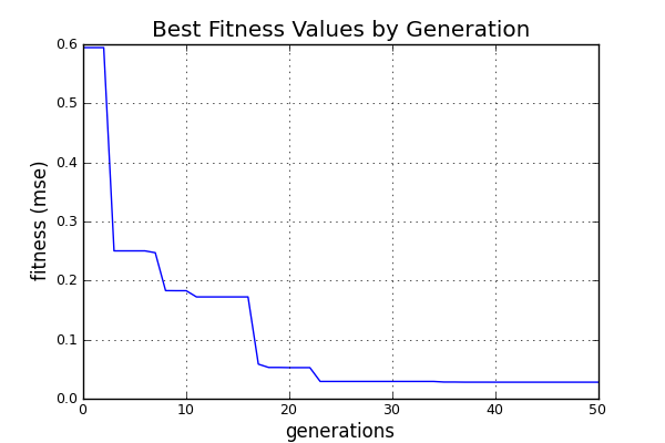
A sample produced: The following is a chart of the best fitness values for each generation. The fitness values rapidly improved until hitting the elbow, followed by a more placid descent.

The actual characteristics of the model generated are as follows:

• Mean Squared Error: 0.0328
• Activation Type: sigmoid
• Hidden Nodes: 5 + 1 bias node
• Learn Rate: 0.4
• Epochs: 300

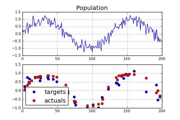
A comparison chart below shows the population and the test samples pulled from the population. While this is toy problem, one might note that the learning set was used solely for computing the appropriate connection weights. The fitness values derived from the validation set. Only the final run of the model used the test data.